A detailed description of Capital Market Assumptions
The Taxficient Score® measures the tax efficiency of a client’s portfolio and the expected after-tax returns projected over a defined period. It is a simple measure of the current tax efficiency of a client’s investments compared to the best and worst-case scenarios. The score allows advisors to introduce the opportunity for maximizing after-tax returns to their clients by optimally locating assets across their IRA and brokerage accounts.
What are Capital Market Assumptions?
Capital Market Assumptions (CMAs) are one of the fundamental data inputs in the calculations of where the assets will be located and directly impacts the Taxficient Score. The CMAs define a set of asset categories to be used, along with referenced investable portfolios (e.g. mutual fund or ETF) on how those asset categories performed in the past. The client’s effective tax rates are used in conjunction with the CMAs to determine optimal asset location for a multi-account investment portfolio.
The applications have four sets of default CMAs, Level 1 (Locked, Customizable) and Level 2 (Locked, Customizable). The Level 1 CMA Set has 6 asset categories and is used for a Quick Proposal. The Level 2 CMA set is more extensive and has 20 asset categories. The (Locked) CMA sets cannot be edited or changed. The (Customizable) CMA sets may be edited to modify, add, change, or delete any categories or their return statistics. These default CMA sets are updated yearly.
Advisors and firms can create their own CMA sets by making changes to the Customizable Sets, or by importing CSV or text files using the import function on the Capital Market Assumptions page.
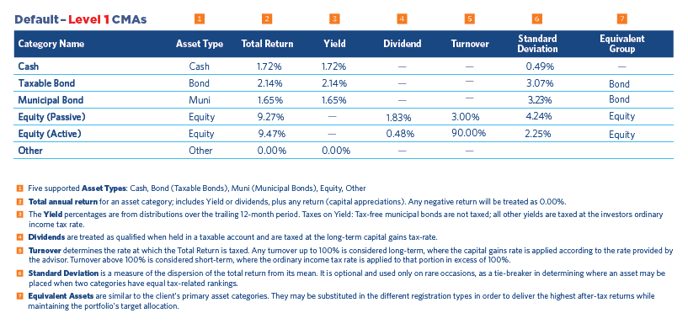
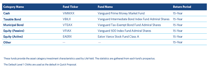
Representative industry-standard funds and ETFs used in LifeYield’s default Level 1 CMAs
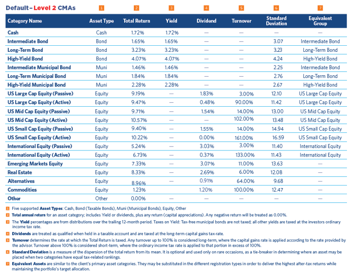
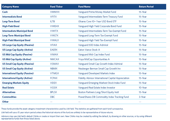
Representative industry-standard funds and ETFs used in LifeYield’s default Level 2 CMAs
How turnover is used in calculating taxes on capital gains
A capital-gains tax is the amount of an asset category’s capital appreciation given up in taxes. The turnover rate is used to determine whether an asset’s capital gains tax is calculated using an investor’s long-term or short-term capital gains rate. A turnover rate of 100% or less is assumed to consist of long-term gain realization. If a turnover rate higher than 100% is specified, then the amount above 100% is treated as short-term gain realization with any remainder being treated as long-term up to a total of 100%.
Examples:
- A turnover rate of 70% would be interpreted as 70% of the category’s capital appreciation being taxed at the long-term capital gains rate, with no taxes being due on the remaining 30%.
- A turnover rate of 140% would be interpreted as 40% of the category’s capital appreciation being taxed at the ordinary income tax rate, combined with 60% (i.e. 100% minus 40%) taxed at the long-term capital gains rate.
- At the two extremes, a turnover rate of 0% implies no capital gains taxes (because nothing is sold, and all gains are deferred beyond the current year), while a turnover rate of 200% implies all capital appreciation is subject to ordinary income tax. Any turnover above 200% will have no impact on the results and is ignored by the formula.
How equivalent categories work
Two or more asset categories may be considered equivalent to each other in terms of meeting an asset allocation. This means that a target allocation containing a category with at least one equivalent can be met with any one of the available equivalents, or even a mix of those categories. It also means that a target allocation containing more than one equivalent asset category is treated in the same way as a target allocation which contains a different mix of the same equivalents. This leads to greater flexibility when meeting a target allocation since a requirement to hold a given target category amount can be met in multiple ways when equivalent categories are available for consideration.
Along with the flexibility in meeting the target allocation, the use of equivalent categories provides an additional opportunity for location optimization, since the same allocation requirement can be met by more than one asset category, and one available category may be better suited to one account type than another. This capability is used to determine the best category to place in each account type to maximize after-tax return.
The two most common applications of equivalents are substituting taxable bonds and municipal bonds that have similar duration and/or substituting active and passive equities that track the same benchmark.